
Dynamic Programming Interview Questions You Must Prepare
Master dynamic programming fundamentals and 10 must-know interview problems with practical techniques, time/space complexities, and optimization tips.

Dynamic programming (DP) is a must-know topic for technical interviews at top companies like Google, Meta, and Amazon. It simplifies complex problems by breaking them into smaller, overlapping subproblems, caching results to improve efficiency. This article explores key DP concepts, problem-solving techniques, and commonly asked interview questions to help you prepare.
Key Takeaways:
- Core Concepts: DP relies on optimal substructure (solutions to subproblems build the larger solution) and overlapping subproblems (reuse computed results).
- Techniques: Learn memoization (top-down recursion with caching) and tabulation (bottom-up iteration) to solve DP problems efficiently.
- Common Indicators: Problems with terms like "maximum", "minimum", "longest", or "number of ways" often involve DP.
Problems Covered:
- Longest Common Subsequence (LCS): Find the longest sequence appearing in the same order in two strings. Applications include DNA analysis and file comparison.
- Longest Increasing Subsequence (LIS): Identify the longest strictly increasing subsequence in an array. Useful in stock trend analysis and scheduling.
- Edit Distance: Calculate the minimum operations (insert, delete, substitute) to transform one string into another. Applied in spell checkers and bioinformatics.
- 0-1 Knapsack Problem: Maximize value within weight constraints. Common in resource allocation and optimization.
- Subset Sum Problem: Determine if a subset of numbers adds up to a target sum. Basis for partitioning and combinatorial problems.
- Coin Change Problem: Find the minimum coins or total combinations to make a specific amount. Relevant in payment systems and vending machines.
- Matrix Chain Multiplication: Optimize the order of matrix multiplication to minimize operations.
- Word Break Problem: Check if a string can be segmented into valid dictionary words. Used in NLP and search engines.
- Rod Cutting Problem: Maximize profit by cutting a rod into smaller pieces based on a price list.
- Fibonacci Sequence: A classic problem demonstrating DP principles, optimized with O(1) space solutions.
Why This Matters:
Mastering DP not only helps you solve interview problems but also builds skills for tackling optimization challenges in full-time jobs. Tools like LeetCode, HackerRank, and Educative.io offer practice problems, while platforms like scale.jobs provide resources like AI resume builders, job application services, and virtual assistants for job seekers to streamline your job search.
Continue reading to dive deeper into problem-solving techniques, examples, and optimization strategies for these essential DP problems.
1. Longest Common Subsequence
Problem Statement and Use Case
The Longest Common Subsequence (LCS) problem involves finding the longest sequence of characters that appears in the same relative order in two strings, though the characters don’t need to be consecutive. For example, given the strings "ABCDGH" and "AEDFHR", the LCS is "ADH" with a length of 3. This problem is a classic example of dynamic programming (DP) principles in action.
LCS has practical applications across various domains. In DNA sequence analysis, it helps compare genetic sequences between organisms. Tools like Git use LCS logic in their diff command to track changes between file versions. Even spell checkers apply LCS variations to measure how closely a misspelled word matches entries in a dictionary. Understanding how DP methods - memoization and tabulation - solve this problem efficiently is crucial.
Dynamic Programming Approach (Top-Down/Bottom-Up)
The key to solving LCS lies in its recurrence relation. If the last characters of two strings match, the LCS length is 1 plus the LCS of their remaining prefixes. If they don’t match, you calculate the maximum of two scenarios: the LCS of the first string with the prefix of the second, or vice versa.
- Memoization uses recursion with caching to store previously computed results, avoiding redundant calculations.
- Tabulation takes an iterative approach, filling a 2D grid where
dp[i][j]represents the LCS of the firsticharacters of string A and the firstjcharacters of string B.
In technical interviews, sketching a recursion tree can help illustrate the repeating subproblems, reinforcing why DP is essential. While memoization is conceptually simpler, tabulation avoids recursion stack overhead and is often preferred in scenarios where performance is critical.
Time Complexity
Both memoization and tabulation achieve a time complexity of O(m × n), where m and n are the lengths of the two input strings. This is a significant improvement over the naive approach, which has an exponential runtime of O(2^max(m, n)). Companies like Google, Amazon, and Meta often test LCS problems because they showcase your ability to transform inefficient solutions into optimized ones - an essential skill in building scalable systems.
Space Complexity and Optimization
The standard DP solution requires O(m × n) space to store the 2D table. However, this can be reduced to O(min(m, n)) by using only two rows instead of the entire matrix. Since each value depends solely on the current and previous rows, this optimization conserves memory. In interviews, discussing this reduced-space approach shows that you’re mindful of resource constraints. Additionally, be ready to explain how to reconstruct the LCS from this optimized structure using backtracking techniques.
2. Longest Increasing Subsequence
Problem Statement and Use Case
The Longest Increasing Subsequence (LIS) problem involves finding the longest subsequence in an array where the elements are strictly increasing. Unlike substrings, the elements in a subsequence don’t need to be consecutive, only in the same relative order. For example, in the array [10, 9, 2, 5, 3, 7, 101, 18], the LIS is [2, 3, 7, 101].
This problem is popular in technical interviews at companies like Microsoft, Facebook, and Bloomberg because it tests your understanding of dynamic programming and optimal substructure principles. Beyond interviews, LIS has practical applications in areas like analyzing stock market trends, optimizing resource allocation in scheduling, and processing time-series data. Even text editors leverage LIS variations to compare document versions and identify stable sections. By solving this, you strengthen your grasp of dynamic programming, setting the stage for tackling more advanced problems.
Dynamic Programming Approach (Top-Down/Bottom-Up)
To solve LIS using dynamic programming (DP), you create a DP array where each element starts at 1, representing the length of the LIS ending at that index. For each index i, you compare it with all previous indices j where arr[j] < arr[i], and update dp[i] using the formula:
dp[i] = max(dp[i], dp[j] + 1).
The final LIS length is the maximum value in the DP array.
For a more efficient solution, you can use a binary search-based method with an auxiliary array. This array keeps track of the smallest possible "tail" elements for increasing subsequences of different lengths. As you iterate through the input, binary search helps determine whether to replace an existing tail or extend the sequence. While this requires a deeper understanding of DP, it significantly reduces time complexity.
Time Complexity
The basic DP solution runs in O(n²) due to the nested loops comparing each element with all previous ones. This approach works well for arrays with a few thousand elements and is often sufficient for interview scenarios. However, the binary search optimization reduces the complexity to O(n log n), making it suitable for processing much larger arrays, such as those with over 100,000 elements. In interviews, you’re typically expected to start with the O(n²) solution and then explain or implement the optimized version when asked.
Space Complexity and Optimization
Both approaches require O(n) space. The standard DP method is easier to implement under time constraints, making it a reliable choice in interviews. Be sure to handle edge cases like empty arrays, duplicate values, and negative numbers. Some interviewers may also ask about variations, such as counting the total number of distinct LIS, which requires tracking additional state alongside the LIS length. Mastering these concepts and techniques will prepare you for other challenging dynamic programming problems often encountered in technical interviews.
Top 5 Dynamic Programming Patterns for Coding Interviews - For Beginners
3. Edit Distance
The Edit Distance problem is a classic example of using dynamic programming (DP) to solve string transformation challenges efficiently.
Problem Statement and Applications
Also known as Levenshtein Distance, this problem calculates the minimum number of operations required to transform one string into another. The allowed operations are: inserting a character, deleting a character, or substituting one character for another. For instance, converting "kitten" to "sitting" takes exactly three steps: replace 'k' with 's', replace 'e' with 'i', and add 'g' at the end.
This problem is a favorite in technical interviews at top companies like Google, Amazon, and Apple. It tests your ability to apply DP principles, such as optimal substructure, to develop efficient solutions. Beyond interviews, Edit Distance has practical uses in spell checkers, DNA sequence alignment in bioinformatics, and natural language processing tasks like machine translation and speech recognition. Mastering this algorithm provides a strong foundation for handling a wide range of string manipulation problems. Let’s break down how DP solves this step by step.
Dynamic Programming Approach: Bottom-Up and Top-Down
The bottom-up approach (tabulation) constructs a 2D table where dp[i][j] represents the edit distance between the first i characters of one string and the first j characters of the other. You start by handling base cases - empty strings, which require adding or removing all characters. From there, the table is filled iteratively: if characters match, take the diagonal value; if they don’t, calculate 1 + min(insert, delete, substitute).
The top-down approach (memoization) uses recursion combined with caching to avoid redundant calculations. While it’s conceptually simpler, the bottom-up method avoids the overhead of recursion, making it more efficient for larger inputs. Both techniques follow the same core logic: if the last characters of the strings match, the distance is the same as their prefixes; otherwise, it’s the minimum of the three operations plus one.
Time Complexity
Both the top-down and bottom-up methods run in O(m × n) time, where m and n are the lengths of the two strings. This is a significant improvement over the naive recursive approach, which has an exponential time complexity of O(3^(m+n)). The DP approach is efficient enough to handle strings with hundreds or even thousands of characters, making it highly practical for both interviews and real-world scenarios.
Space Complexity and Optimizations
The standard tabulation method requires O(m × n) space to store the DP table. However, this can be optimized to O(min(m, n)) using rolling arrays, as each row in the table depends only on the previous one. This optimization is particularly helpful when working with very long strings.
It’s also worth exploring related concepts, such as Hamming Distance (which considers only substitutions for strings of equal length) and Damerau-Levenshtein Distance (which includes transpositions of adjacent characters). These variations build on the fundamentals of Edit Distance and introduce new challenges for advanced DP problems.
4. 0-1 Knapsack Problem
Problem Statement and Use Case
The 0-1 Knapsack Problem is a well-known optimization challenge where the goal is to maximize the total value of items that can fit into a knapsack with a fixed weight capacity. The "0-1" aspect means you must either take an item entirely or leave it out - there's no option to take fractions of an item. This makes it distinct from the Fractional Knapsack Problem, which can be solved with a greedy approach since items can be divided.
This problem is a staple in technical interviews at companies like Google, Amazon, and Microsoft because it tests your ability to identify optimal substructure and overlapping subproblems - key concepts in dynamic programming (DP). Beyond interviews, it has practical applications in areas like resource allocation, trip packing, and system design optimization. A common mistake is applying a greedy approach here, which only works for the Fractional Knapsack Problem. Instead, the problem's structure lends itself naturally to a DP solution.
Dynamic Programming Approach (Top-Down and Bottom-Up)
The bottom-up approach uses a 2D table where dp[i][w] represents the maximum value you can achieve using the first i items with a weight limit of w. The process begins with base cases - if there are no items or the capacity is zero, the maximum value is zero. From there, the table is filled iteratively. For each item, you decide whether to include it or exclude it:
- If the item's weight exceeds the current capacity, it cannot be included.
- Otherwise, you calculate the maximum value by comparing the result of including the item (adding its value to the result for the remaining capacity) and excluding it.
The top-down approach (using memoization) relies on recursion to explore both options - include or exclude each item - and stores computed results in a 2D array or hashmap. While this approach is easier to conceptualize, the bottom-up method avoids recursion overhead and simplifies space optimization. The recurrence relation for both approaches is:
dp[i][w] = max(value[i] + dp[i-1][w - weight[i]], dp[i-1][w])
This applies only if the item's weight does not exceed the current capacity.
Time Complexity
Both the top-down and bottom-up approaches have a time complexity of O(N × W), where N is the number of items and W is the knapsack's weight capacity. This is a massive improvement compared to the brute-force recursive solution, which has an exponential complexity of O(2^N). For instance, with just 4 items, a brute-force approach could require 31 recursive calls, making it infeasible for larger inputs.
Space Complexity and Optimization
The traditional DP table requires O(N × W) space. However, since each row depends only on the previous row, this can be optimized to O(W) by using a single-dimensional array. When implementing this optimization, it’s crucial to iterate through the weight capacity in reverse order (from W down to the item's weight). This ensures that each item is only considered once per iteration, avoiding errors that would turn the problem into an Unbounded Knapsack Problem.
If you need to reconstruct the list of selected items rather than just calculate the maximum value, you'll need to maintain a full 2D table or use a separate array to track choices. Mastering the 0-1 Knapsack Problem not only prepares you for technical interviews but also sharpens your ability to solve optimization problems in practical scenarios.
5. Subset Sum Problem
Problem Statement and Use Case
The Subset Sum Problem is a classic decision-making challenge in dynamic programming. It asks whether there is a subset within a given set of integers that adds up to a specific target sum. For instance, consider the set {3, 34, 4, 12, 5, 2} with a target sum of 9. The task is to determine if any combination of numbers from the set equals 9. In this case, the subset {4, 5} satisfies the condition.
This problem is a staple in technical interviews at companies like Amazon, Microsoft, and Google, as it tests your grasp of dynamic programming principles. It also lays the groundwork for related problems, such as Partition Equal Subset Sum and Count of Subsets with a Given Sum.
Dynamic Programming Approach (Top-Down and Bottom-Up)
To solve the Subset Sum Problem, you decide for each element whether to include it in the subset or exclude it. This decision is captured in the recurrence relation:
isSum(i, target) = isSum(i-1, target) OR isSum(i-1, target - set[i]).
Here, the solution depends on whether the current element is excluded or included.
Bottom-Up Approach
The bottom-up method uses a 2D table dp[i][j], where each cell represents whether a sum j can be achieved using the first i elements. The process starts with base cases - an empty subset can only form a sum of zero - and iteratively fills the table.
Top-Down Approach
The top-down method relies on recursion with memoization. It begins with the target sum and works backward to smaller subproblems, storing results in a cache to avoid redundant calculations. This approach closely mirrors the recurrence relation, making it easier to visualize.
Comparing the Two Approaches
| Feature | Top-Down (Memoization) | Bottom-Up (Tabulation) |
|---|---|---|
| Method | Recursive | Iterative |
| Direction | Starts with the target and drills down to base cases | Starts with base cases and builds up to the target |
| Implementation | Intuitive, as it follows the recursive relation | Easier to optimize for space |
| State Space | Computes only required states | Computes all states in the table |
Time Complexity
Both approaches achieve a time complexity of O(N × S), which is a significant improvement over the exponential time of the brute-force method.
Space Complexity and Optimization
The standard DP table requires O(N × S) space. However, since each row depends only on the previous row, you can reduce the space requirement to O(S) by using a single-dimensional array. To implement this optimization, iterate through the target sum in reverse order to ensure each element is processed only once per iteration.
6. Coin Change Problem
Problem Statement and Use Case
The Coin Change Problem revolves around finding the minimum number of coins needed to make a specific amount, given an unlimited supply of coins in various denominations. For instance, with coins of {1, 5, 10, 25} cents, you can make 63 cents using six coins: two 25¢ coins, one 10¢ coin, and three 1¢ coins.
This problem is a staple in coding interviews and has practical applications in areas like vending machine algorithms, payment systems, and currency exchange software. It typically appears in two forms: determining the minimum number of coins required (optimization) and calculating the total number of ways to make the target amount (combinatorics).
Dynamic Programming Approach (Top-Down and Bottom-Up)
The key idea behind solving this problem lies in breaking it into smaller subproblems. For any given amount, you evaluate each coin denomination using the recurrence relation:
minCoins(amount) = 1 + min(minCoins(amount - coin))
This approach exemplifies the divide-and-conquer principle at the heart of dynamic programming (DP).
Bottom-Up Approach
The bottom-up method involves creating a DP array where each entry, dp[i], represents the minimum number of coins needed to make the amount i. Starting with the base case dp[0] = 0, you iterate through amounts from 1 to the target, updating dp[i] by considering each coin denomination. For every amount, the formula dp[i] = min(dp[i], 1 + dp[i - coin]) ensures you find the optimal solution.
Top-Down Approach
The top-down approach uses recursion combined with memoization. Starting from the target amount, the algorithm recursively computes solutions for smaller amounts. When the amount reaches 0, the function returns 0 as the base case. Memoization stores previously calculated results, preventing redundant computations and significantly improving efficiency.
| Feature | Top-Down (Memoization) | Bottom-Up (Tabulation) |
|---|---|---|
| Mechanism | Recursive + Cache | Iterative DP Table |
| Time Complexity | O(amount × Number of Coins) | O(amount × Number of Coins) |
| Space Complexity | O(amount) + Recursion Stack | O(amount) |
Time Complexity
Both approaches achieve a time complexity of O(amount × Number of Coins). This is a substantial improvement compared to the brute-force recursive method, which has exponential complexity and quickly becomes infeasible for larger inputs.
Space Complexity
The space requirements differ slightly between the two approaches. The bottom-up method uses O(amount) space for the DP array. On the other hand, the top-down approach also requires O(amount) space for memoization but adds extra space for the recursion call stack, which can grow to O(amount) in the worst-case scenario. This makes the bottom-up approach slightly more space-efficient overall.
7. Matrix Chain Multiplication
Problem Statement and Use Case
Matrix Chain Multiplication focuses on finding the most efficient way to multiply a sequence of matrices. While matrix multiplication is associative - meaning the order of operations can change without affecting the result - the number of scalar multiplications required depends heavily on how the matrices are parenthesized.
Take this example: matrices A (10×30), B (30×5), and C (5×60). If you compute ((AB)C), the cost is 4,500 operations, while calculating (A(BC)) requires 27,000 operations - a massive difference. This problem is not just a theoretical exercise; it has practical applications, such as optimizing database queries where determining the best order for join operations can significantly reduce computational effort. It’s also a common topic in technical interviews, especially when discussing dynamic programming (DP), making it a must-know for candidates. Utilizing free job application tools can further streamline your preparation process.
Dynamic Programming Approach (Top-Down and Bottom-Up)
A brute-force solution to this problem is impractical due to its exponential time complexity. Dynamic programming offers an efficient way to solve it by leveraging two fundamental properties:
- Optimal substructure: The best solution for the entire chain depends on the best solutions for its smaller sub-chains.
- Overlapping subproblems: Naive recursion ends up recalculating costs for the same sub-chains multiple times.
To implement the DP solution, you create a 2D table (m[i, j]), where (m[i, j]) represents the minimum cost to multiply matrices from (i) to (j). For every possible split (k), calculate:
[ m[i, j] = m[i, k] + m[k+1, j] + (\text{rows}_i \times \text{cols}_k \times \text{cols}_j) ]
Start with the base case where (i = j) (a single matrix has no multiplication cost). Then, solve for chains of increasing lengths, working up to the full sequence. To reconstruct the optimal parenthesization, maintain a separate table to store the split points. This is often an additional requirement in interviews.
The top-down approach uses recursion with memoization, computing subproblems only as needed. On the other hand, the bottom-up approach builds the solution iteratively using tabulation. Both methods avoid redundant calculations, but the bottom-up approach is often preferred for its simplicity and resilience against stack overflow errors in deep recursion scenarios.
Time Complexity
The time complexity of the dynamic programming solution is O(n³). This comes from the three nested loops: one iterating over chain lengths, another over starting indices, and the last testing all possible split points (k). Compared to the exponential complexity of brute force, this is a significant improvement and well-suited for interview discussions.
Space Complexity and Optimization
Both the top-down and bottom-up approaches require O(n²) space to store the cost table and the split table for all sub-chains. The top-down method uses additional space for recursion, while the bottom-up approach avoids this, making it more memory-efficient for long chains. Storing the split table is essential for reconstructing the parenthesization, which is often part of the problem requirements.
In production scenarios, the bottom-up method is generally favored for its straightforward implementation and reduced risk of stack overflow. Understanding these nuances and optimizations ensures clarity and efficiency in both coding interviews and practical applications.
8. Word Break Problem
Problem Statement and Use Case
The Word Break Problem is a classic example of how dynamic programming (DP) can simplify complex string problems by avoiding redundant calculations. The task is simple in theory: determine if a given string can be segmented into valid words from a dictionary. For instance, if the dictionary contains {"leet", "code"} and the string is "leetcode", the answer is yes, as it can be split into "leet" and "code". However, with the string "leetcodes" and the same dictionary, the answer would be no.
This problem often shows up in technical interviews and is typically rated as Medium to Hard in difficulty. Beyond interviews, it has practical applications in areas like natural language processing, autocorrect systems, and search query parsing. For example, when you type a phrase without spaces into a search engine, algorithms similar to the Word Break Problem help identify whether the input can be matched to valid words or terms. Like other DP problems, this challenge focuses on dividing the task into smaller, overlapping subproblems that can be solved efficiently.
Dynamic Programming Approach (Top-Down and Bottom-Up)
Both the top-down and bottom-up DP methods rely on the idea of optimal substructure: if a valid prefix of the string exists, the remaining part of the string must also be segmentable for the solution to work. A naive recursive approach would repeatedly process the same suffixes, leading to inefficiency. DP tackles this by caching results and avoiding duplicate work.
-
Bottom-Up Approach: This method uses a boolean array
dp[i], wheredp[i]istrueif the firsticharacters of the string can be segmented. Start withdp[0] = true(an empty string is always valid). For each positioni, check all previous indicesjwheredp[j]istrueand the substring fromjtoiexists in the dictionary. - Top-Down Approach: This method leverages recursion with memoization. It stores results for each suffix in a hashmap, ensuring that no suffix is processed more than once. A HashSet is typically used for dictionary lookups, enabling O(1) time complexity for checking if a substring is a valid word.
Time Complexity
The time complexity for these approaches is O(n²), as each substring is checked against the dictionary. Using a Trie for the dictionary can improve efficiency by reducing redundant character comparisons, but the overall complexity remains O(n²).
Space Complexity and Optimization
The space complexity is O(n) for the DP array, with an additional O(n) space required for recursion in the top-down approach. In some variations of this problem, such as Word Break II, you may be asked to return all possible segmentations. This introduces backtracking, which significantly increases both time and space complexity due to the need to explore multiple valid combinations.
9. Rod Cutting Problem
Problem Statement and Use Case
The rod cutting problem is a classic dynamic programming challenge that focuses on finding the best way to maximize revenue by cutting a rod into smaller pieces. You're given a rod of length n and a price list that specifies the value of each possible cut. The task is to decide where to make cuts - or whether to leave the rod intact - to achieve the highest profit. For instance, if you have a rod of length 4 and a price list [1, 5, 8, 9] (for lengths 1 through 4), cutting the rod into two pieces of length 2 results in a total of $10, which is higher than the $9 you'd get without making any cuts.
This problem is a staple in dynamic programming interview questions, ranking among the top 20. It tests your ability to recognize and leverage two key principles of dynamic programming: optimal substructure and overlapping subproblems. These concepts pave the way for implementing both bottom-up and top-down approaches. Beyond interviews, the logic behind this problem has practical applications in tasks like optimizing material usage in manufacturing.
Dynamic Programming Approach (Top-Down and Bottom-Up)
The core idea lies in the concept of optimal substructure. For a rod of length n, the maximum revenue can be calculated as the sum of the revenue from the best first cut of length i and the maximum revenue from the remaining piece of length n-i. A straightforward recursive approach, however, recalculates the same subproblems multiple times, leading to exponential time complexity.
-
Bottom-Up Approach: This method builds solutions iteratively, starting with the smallest rod lengths and working upward. You use an array
dp[i], wheredp[i]stores the maximum revenue for a rod of length i. Begin by initializingdp[0] = 0, then, for each rod length, evaluate all possible first cuts to determine the maximum revenue. This approach avoids the overhead of recursive calls and is often preferred in real-world applications due to its efficiency and stability. - Top-Down Approach: This method employs recursion with memoization. Starting with the full rod length, you recursively explore all possible cuts while storing previously computed results in a cache to avoid redundant calculations. Although this method only solves the necessary subproblems, it carries the risk of recursion stack overflow for very large inputs, making it less suitable for production use.
Time Complexity
Both the top-down and bottom-up approaches share a time complexity of O(n²). This arises because, for each rod length from 1 to n, you evaluate all possible first cuts, resulting in approximately n²/2 operations. This complexity is similar to other dynamic programming problems like the 0-1 Knapsack problem.
Space Complexity and Optimization
The space complexity for both approaches is O(n), as they rely on an array to store intermediate results. The top-down method, however, requires additional O(n) space for the recursion call stack, making it slightly less efficient. For large inputs, the bottom-up approach is generally preferred since it avoids the risk of stack overflow. Further space optimization isn't possible here, as each computation depends on all preceding values, making the use of the entire array essential.
10. Fibonacci Sequence
Problem Statement and Use Case
The Fibonacci Sequence is a classic example of dynamic programming (DP), showcasing the principles of overlapping subproblems and optimal substructure. It’s a series where each number is the sum of the two preceding ones, starting with 0 and 1. Mathematically, it’s defined as F(n) = F(n-1) + F(n-2), with the base cases being F(0) = 0 and F(1) = 1.
In technical interviews, this problem is often used to evaluate your ability to identify and eliminate redundant computations in naive recursive solutions. A naive recursive approach recalculates Fibonacci numbers multiple times, leading to an exponential time complexity of O(2^n). For instance, computing F(5) involves solving F(3) three times and F(2) five times, making it inefficient for larger inputs like n = 40.
Dynamic Programming Approach (Top-Down and Bottom-Up)
Top-Down (Memoization)
This approach uses recursion combined with caching. Results are stored in a cache, such as an array or hashmap, so when the function is called for F(n), it first checks the cache. If the value is already calculated, it’s returned in constant time (O(1)), avoiding redundant computations. This method starts from the target value and works backward to the base cases, making it intuitive for those familiar with recursion.
Bottom-Up (Tabulation)
In this method, the solution is built iteratively from the base cases up to n. An array is used to store Fibonacci numbers, with each index holding the value of the corresponding Fibonacci number. The value at index i is computed as the sum of the values at i-1 and i-2. This approach avoids the overhead of recursion, making it more efficient and suitable for production environments.
Time Complexity
Both memoization and tabulation reduce the time complexity from exponential O(2^n) to linear O(n). Each Fibonacci number is computed only once, with a single addition performed for each of the n steps.
Space Complexity and Optimization
The standard implementations of both memoization and tabulation require O(n) space. Memoization needs space for the cache and the recursion stack, while tabulation uses an array to store intermediate results. However, the bottom-up approach can be optimized to use O(1) space by maintaining only the last two Fibonacci numbers in variables, eliminating the need for an array. This space-efficient version is a common interview follow-up question, testing your ability to refine a solution further.
| Approach | Time Complexity | Space Complexity | Description |
|---|---|---|---|
| Naive Recursion | O(2^n) | O(n) (stack) | Recomputes values multiple times due to redundant calculations. |
| Memoization (Top-Down) | O(n) | O(n) | Uses recursion with caching to avoid redundant computations. |
| Tabulation (Bottom-Up) | O(n) | O(n) | Iteratively builds the solution from base cases using an array. |
| Space-Optimized DP | O(n) | O(1) | Uses two variables instead of an array to achieve constant space usage. |
Problem Complexity Comparison Table
Dynamic Programming Problems: Time and Space Complexity Comparison
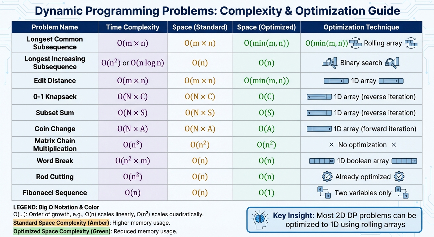
Understanding complexity patterns and optimization methods in dynamic programming is a key skill for solving these problems effectively. Below is a table summarizing the time and space complexities of common dynamic programming problems, along with their space-saving techniques.
| Problem | Time Complexity | Space Complexity (Standard) | Space Complexity (Optimized) | Optimization Technique |
|---|---|---|---|---|
| Longest Common Subsequence | O(m × n) | O(m × n) | O(min(m, n)) | Rolling array (store only current and previous row) |
| Longest Increasing Subsequence | O(n²) or O(n log n) | O(n) | O(n) | Binary search for O(n log n) time |
| Edit Distance | O(m × n) | O(m × n) | O(min(m, n)) | 1D array with forward iteration |
| 0-1 Knapsack Problem | O(N × C) | O(N × C) | O(C) | 1D array with downward capacity iteration |
| Subset Sum Problem | O(N × S) | O(N × S) | O(S) | 1D array with downward sum iteration |
| Coin Change Problem | O(N × A) | O(N × A) | O(A) | 1D array with upward amount iteration (unbounded) |
| Matrix Chain Multiplication | O(n³) | O(n²) | O(n²) | No common space optimization; full table required |
| Word Break Problem | O(n² × m) | O(n) | O(n) | Efficient with 1D boolean array |
| Rod Cutting Problem | O(n²) | O(n) | O(n) | Already optimized with 1D array (unbounded knapsack) |
| Fibonacci Sequence | O(n) | O(n) | O(1) | Store only the last two values in variables |
Key Insights for Optimization
- Two-Dimensional State Problems: Problems like Longest Common Subsequence (LCS) and Edit Distance often have O(m × n) space complexity due to their 2D tables. However, these can be reduced to O(min(m, n)) by using rolling arrays. As Yangshun Tay, a former Meta Staff Engineer, explains:
"Sometimes you do not need to store the whole DP table in memory; the last two values or the last two rows of the matrix will suffice."
- Knapsack-Style Problems: For problems like 0-1 Knapsack, the direction of iteration matters when using a 1D array. Iterating downward for capacity ensures that each item is used only once, which is critical to avoid logical errors.
-
Understanding Time Complexity: Dynamic programming time complexity is determined by the number of states multiplied by the transition cost. For instance:
- Edit Distance: m × n states with constant-time transitions result in O(m × n) time.
- Matrix Chain Multiplication: O(n²) states, each requiring O(n) work to find the optimal split point, lead to O(n³) time.
- 1D Array Optimization: When dp[i][j] relies only on dp[i–1], you can often replace the 2D table with a 1D array to save space. Recognizing this dependency is crucial for applying optimizations quickly during interviews.
Conclusion
Becoming proficient in dynamic programming (DP) is a key step for anyone aiming to excel in technical interviews at top tech companies. These questions are designed to test not just your coding skills but also your ability to break down complex problems and create efficient solutions. The ability to identify overlapping subproblems and transform exponential solutions into linear or polynomial time is what sets standout candidates apart.
The examples of DP challenges discussed earlier highlight the specific skills you'll need to refine. However, true mastery comes from consistent, hands-on practice - not from simply memorizing solutions. As LeetCode wisely puts it:
"Deliberate practice does not mean looking for answers and memorizing it. You won't go very far with that approach."
To truly improve, tackle these problems repeatedly. By your third or fourth attempt, you'll notice your code becoming more concise and efficient, as you'll uncover optimization strategies you might have missed initially. This kind of deliberate, focused practice lays the groundwork for success.
To aid your preparation, platforms like LeetCode and HackerRank provide excellent resources. LeetCode’s "Top Interview Questions" collection includes foundational DP problems like Climbing Stairs and Maximum Subarray, while HackerRank’s Interview Preparation Kit features a dedicated section on dynamic programming. For a deeper understanding of patterns, Educative.io’s Grokking Dynamic Programming Patterns course is a great resource for learning to identify problem structures instead of memorizing solutions.
Once your technical skills are polished, the next challenge is making your job application stand out. This is where scale.jobs can help. The platform offers free tools like an Interview Questions Predictor, which analyzes job postings to forecast likely questions, and an ATS Resume Checker to ensure your application clears automated screening systems. For more tailored support, their AI Assistant Pro ($9/month) generates unlimited custom resumes and cover letters, while their Human Assistant service ($199–$1,099) provides trained virtual assistants to handle job applications, saving you over 20 hours a week - time you can use to focus on interview prep and networking.
FAQs
What’s the difference between memoization and tabulation in dynamic programming?
Memoization works as a top-down approach, where the algorithm begins with the main problem and divides it into smaller, manageable subproblems. As the function tackles these subproblems, it stores the results of recursive calls in a cache, but only when needed. This way, it avoids recalculating solutions for problems it has already solved.
Tabulation takes a different path with a bottom-up approach. Instead of waiting for subproblems to arise, it solves all possible subproblems in advance using an iterative process. These solutions are stored in a table, and the method gradually builds up to the solution of the main problem, starting from the simplest cases.
To put it simply, memoization solves problems on demand, while tabulation prepares solutions ahead of time.
How do I know if a problem can be solved using dynamic programming?
Dynamic programming works best for problems that can be divided into smaller, overlapping subproblems and exhibit an optimal substructure. Essentially, this means you can solve a larger problem by efficiently combining solutions to its smaller parts. If you notice patterns involving recursion or repeated calculations, it’s a strong indicator that dynamic programming could simplify and speed up the process.
What are the best strategies to reduce space complexity in dynamic programming problems?
Reducing the space complexity in dynamic programming (DP) is all about trimming down the extra memory needed while still being able to reuse previously computed results. Since DP often involves storing solutions to subproblems, memory usage can balloon quickly if a full table is used. Here are a few practical ways to optimize space:
- Rolling arrays: If your recurrence only depends on the previous row or column, you can simplify things by using a single 1-D array or just two alternating rows. This approach overwrites data as you iterate, cutting down space requirements from O(n × m) to O(min(n, m)).
- Sparse memoization: Instead of creating an entire matrix, you can use a hash map or dictionary to store only the states you actually calculate. This is especially handy when dealing with problems that have large state spaces but only a small portion of them are visited.
- State compression: For variables that are binary or have small, bounded ranges, you can combine multiple dimensions into a single integer or use a bitset. This compactly represents states and saves memory.
These strategies are particularly useful for tackling classic problems like Longest Common Subsequence, knapsack, or coin change. They not only help you work within memory limits but also make your solutions more efficient - something that’s often crucial in technical interviews.